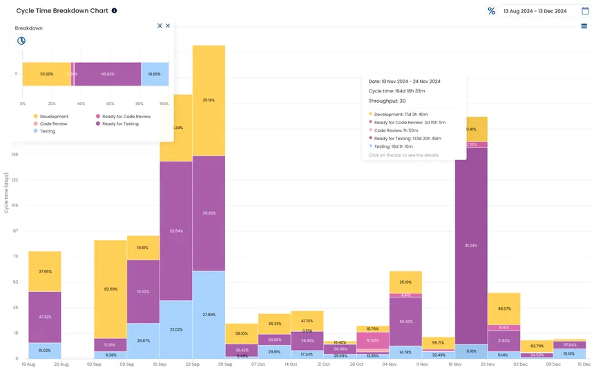
Cycle Time Breakdown
Open this chart to investigate outliers, the work items on the tail of the distribution that took significantly longer to finish.
What it answers
How long does work take?
Understand the distribution of historical cycle times and the likelihood of completing similar work within a given time.
Example

Read each bar against the vertical frequency axis and the horizontal cycle time axis to understand the frequency distribution of task completion times.
A percentile line shows the probability of completing tasks within a certain cycle time. Higher percentile lines indicate a higher likelihood of delivering work on time.
The Cycle Time Averages widget shows the mean, median and mode average cycle times and how their trends develop over time.
The Cycle Time Histogram shows how often tasks are completed at each cycle time. The vertical axis shows frequency, and the horizontal axis shows cycle time.
Use the distribution to determine how much your cycle time varies.
A large hump on the left followed by a long tail to the right indicates significant variation and an inconsistent process. Consider establishing a WIP-limited pull system to work toward more predictable delivery times.

The Cycle Time Histogram uses past cycle time data to forecast likely delivery times.
Percentile lines show the probability of completing tasks within a certain cycle time. Higher percentiles indicate a higher likelihood of delivering work on time.
Use percentile lines to define your service level agreements. Discuss confidence levels with clients and stakeholders, then base your SLAs on their optimum comfort level. We recommend starting with the 85th percentile line.

Average cycle time is a measure of performance. The Cycle Time Histogram shows your mean, median and mode average cycle times and how they change over time.
Ideally, these lines should remain close together and either stay level or go down.
Choose an average and monitor its line. If it rises, your team needs more time, on average, to complete tasks. You might need to reevaluate your WIP limits or alter your process policies to establish a faster delivery workflow.

You can export the filtered data shown in this chart as a CSV.
A large hump on the left followed by a long tail to the right indicates significant cycle time variation and an inconsistent process.
Two peaks form a bimodal distribution, indicating that two groups overlap in the dataset.
Divide the 98th percentile by the 50th percentile. A result of 5.6 or more indicates a fat-tailed frequency distribution and helps determine whether you can rely on the probability forecast.
Open this chart to investigate outliers, the work items on the tail of the distribution that took significantly longer to finish.
Connect your existing delivery data and start exploring your flow.